Bmk_Space_mapping.R Operating Instructions

1. Open the script file

source(‘xxx’) #’xxx’ is the script path, for example ’C:/Users/R/Desktop/qq.R’

2. Create a Seurat object and plot the spatial cluster map

FilePath : folder path containing “barcode.tsv.gz, barcode_pos.tsv.gz, feature.tsv.gz, matrix.mtx.gz”
barcode_pos_file : file path of “barcode_pos.tsv.gz”
out_path : output file directory
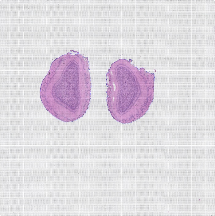
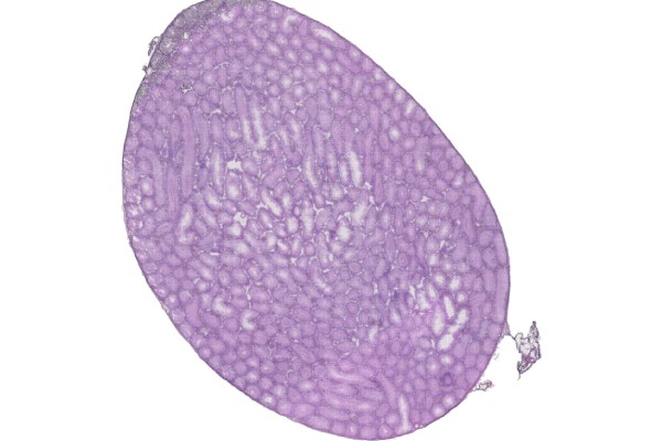
png_path : HE staining image (.png format). If the file is in .tiff format it must be converted; note that the resolution can be reduced during conversion to avoid read failures caused by an excessively large .png file
Note that the Seurat object must be named “object”

object <- Create_object(

FilePath = ‘E:/AAAWork/BSTViewer_project/subdata/L13_heAuto/’,

barcode_pos_file = ‘E:/AAAWork/BSTViewer_project/subdata/L13_heAuto/barcodes_pos.tsv.gz’,

out_path = ‘C:/Users/R/Desktop/temp/Cluster/’,

png_path = ‘C:/Users/R/Desktop/temp/he.png’,

min.cells = 10, # A gene is retained only if expressed in at least n cells; adjustable, default 10

min.features = 100, # A cell is retained only if it has at least n genes; adjustable, default 100

dims = 1:30, # Number of PCs used for downstream analysis; adjustable, default 1:30

resolution = 0.5, # Sets the “granularity” of downstream analysis; higher values yield more clusters; adjustable, default 0.5

point_size = 3, # Point size; adjust according to the matrix file level — the smaller the level, the smaller the value

width = 12, # Width of the output image; adjustable, default 12

height = 5, # Height of the output image; adjustable, default 5

Cluster = T, # Whether to perform clustering analysis; default F

label = T # Whether to output a labeled cluster plot

)

umap_cluster_label

3. UMI statistics

object <- Create_object(

FilePath = ‘E:/AAAWork/BSTViewer_project/subdata/L13_heAuto/’,

barcode_pos_file = ‘E:/AAAWork/BSTViewer_project/subdata/L13_heAuto/barcodes_pos.tsv.gz’,

out_path = ‘C:/Users/R/Desktop/temp/UMI_stat/’,

png_path = ‘C:/Users/R/Desktop/temp/he.png’,

point_size = 3, # Same as above

width = 12, # Same as above

height = 5, # Same as above

UMI_stat = T) # Whether to compute UMI statistics

UMI_viol_heatmap

4. nFeature statistics

object <- Create_object(

FilePath = ‘E:/AAAWork/BSTViewer_project/subdata/L13_heAuto/’,

barcode_pos_file = ‘E:/AAAWork/BSTViewer_project/subdata/L13_heAuto/barcodes_pos.tsv.gz’,

out_path = ‘C:/Users/R/Desktop/temp/Gene_stat/’,

png_path = ‘C:/Users/R/Desktop/temp/he.png’,

point_size = 2, # Same as above

width = 12, # Same as above

height = 5, # Same as above

nFeature_stat = T) # Whether to compute nFeature statistics

nFeature_viol_heatmap

5. Output the marker genes of each cluster and plot the expression heatmap of individual genes

object <- Create_object(

FilePath = ‘E:/AAAWork/BSTViewer_project/subdata/L13_heAuto/’,

barcode_pos_file = ‘E:/AAAWork/BSTViewer_project/subdata/L13_heAuto/barcodes_pos.tsv.gz’,

out_path = ‘C:/Users/R/Desktop/temp/Single_gene_1/’,

png_path = ‘C:/Users/R/Desktop/temp/he.png’,

point_size = 2, # Same as above

Gene_stat = T, # Whether to plot marker genes

top_gene = 1, # Number of top marker genes taken per cluster; adjustable, but the value should not be set too large

min.pct = 0.25, # Minimum fraction of cells in which a gene must be expressed in any two cell groups; adjustable

logfc.threshold = 0.25, # Fold-change threshold; adjustable

markpic_width = 8, # Width of the violin plot and tSNE plot

markpic_height = 12, # Height of the violin plot and tSNE plot

)

Heatmap list

6. Plot the cluster map of one or several genes

object <- Create_object(

FilePath = ‘E:/AAAWork/BSTViewer_project/subdata/L13_heAuto/’,

barcode_pos_file = ‘E:/AAAWork/BSTViewer_project/subdata/L13_heAuto/barcodes_pos.tsv.gz’,

out_path = ‘C:/Users/R/Desktop/temp/Test/Single_gene_2/’,

png_path = ‘C:/Users/R/Desktop/temp/he.png’,

point_size = 2.6, # Same as above

Gene_stat = T, # Whether to plot marker genes

Custom_gene = T, # Whether to plot custom genes

alpha_continuous = c(0.5,1) # Adjust the transparency range according to gene expression

gene_list = c(‘Hpca’)) # Names of the genes to plot; multiple genes can be entered

Hpca

Select a black background for highlighting

object <- Create_object(

FilePath = ‘E:/AAAWork/BSTViewer_project/subdata/L13_heAuto/’,

barcode_pos_file = ‘E:/AAAWork/BSTViewer_project/subdata/L13_heAuto/barcodes_pos.tsv.gz’,

out_path = ‘C:/Users/R/Desktop/temp/Test/Single_gene_2/’,

png_path = ‘C:/Users/R/Desktop/temp/he.png’,

point_size = 2.6, # Same as above

Gene_stat = T, # Whether to plot marker genes

Custom_gene = T, # Whether to plot custom genes

dark_background = T, # Black background

gene_list = c(‘Hpca’)) # Names of the genes to plot; multiple genes can be entered

Hpca

7. Plot a single cluster

object <- Create_object(

FilePath = ‘E:/AAAWork/BSTViewer_project/subdata/L13_heAuto/’,

barcode_pos_file = ‘E:/AAAWork/BSTViewer_project/subdata/L13_heAuto/barcodes_pos.tsv.gz’,

out_path = ‘C:/Users/R/Desktop/temp/TestL6/single/’,

png_path = ‘C:/Users/R/Desktop/temp/he.png’,

point_size = 2, # Same as above

Single_cluster = T # Whether to plot a single cluster

)

cluster1

Single cluster list