
BSTMatrix v2.3: R Environment Setup, Installation and User Guide
Warning: Trying to access array offset on value of type bool in /www/wwwroot/10.3.128.39/wp-content/themes/betheme/functions/theme-functions.php on line 1338
Warning: Trying to access array offset on value of type bool in /www/wwwroot/10.3.128.39/wp-content/themes/betheme/functions/theme-functions.php on line 1343
Warning: Trying to access array offset on value of type bool in /www/wwwroot/10.3.128.39/wp-content/themes/betheme/functions/theme-functions.php on line 1365
Warning: Trying to access array offset on value of type bool in /www/wwwroot/10.3.128.39/wp-content/themes/betheme/functions/theme-functions.php on line 1366
Warning: Trying to access array offset on value of type bool in /www/wwwroot/10.3.128.39/wp-content/themes/betheme/functions/theme-functions.php on line 1367
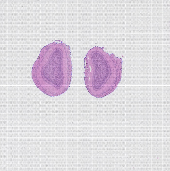
BMKManu DG1000 — Brain Nuclei of a Wild Animal
2022-05-31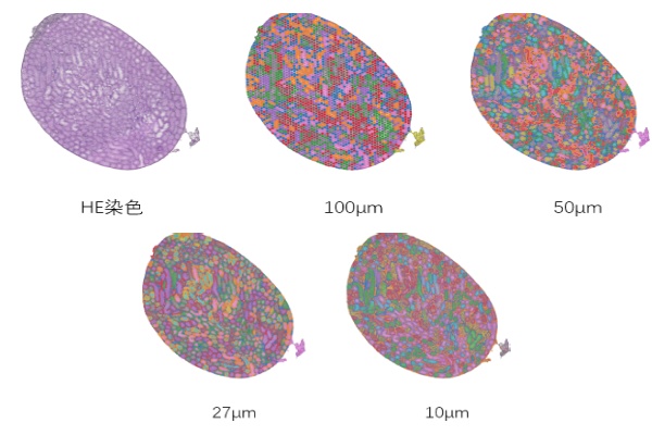
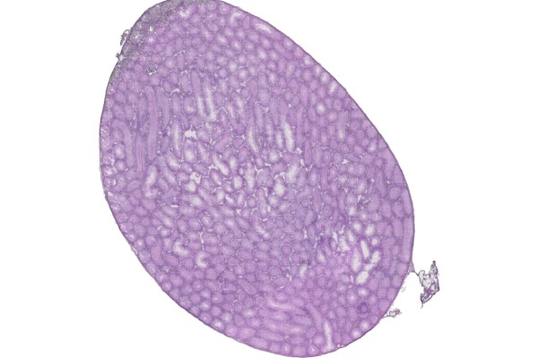
BSTViewer v3.0 Installation Tutorial
2022-06-08Warning: Trying to access array offset on value of type bool in /www/wwwroot/10.3.128.39/wp-content/themes/betheme/functions/theme-functions.php on line 1338
Warning: Trying to access array offset on value of type bool in /www/wwwroot/10.3.128.39/wp-content/themes/betheme/functions/theme-functions.php on line 1343
Warning: Trying to access array offset on value of type bool in /www/wwwroot/10.3.128.39/wp-content/themes/betheme/functions/theme-functions.php on line 1365
Warning: Trying to access array offset on value of type bool in /www/wwwroot/10.3.128.39/wp-content/themes/betheme/functions/theme-functions.php on line 1366
Warning: Trying to access array offset on value of type bool in /www/wwwroot/10.3.128.39/wp-content/themes/betheme/functions/theme-functions.php on line 1367
Generate Matrix
1.1 Software Environment Dependencies
A)python: version 8 or above, with the cv2 module installed (4.0 or above), matplotlib, seaborn, pandas (1.5.0 or above), tifffile, Cellpose, Pyyaml, scikit-image, tqdm
B) Star: version 6.1d or above
C) perl: the threads and threads::shared modules
D) Rscript: the following R packages are required — seurat, dplyr, tibble, ggplot2, broom, purrr, cowplot, cluster, ggpubr, plotly, htmlwidgets, kableextra, htmltools, shiny, knitr, rmarkdown, optparse, getopt.
E)Pandoc.
[The dependent software must be added to the environment variables with export so that the pipeline can invoke it.]
[For environment deployment, refer to the file “Environment_Configuration.rst” in the installation directory.]
1.2 Input Data
A) Sequencing data: paired-end FASTQ data.
B) Reference genome data: genome sequence file, GTF file (column 3 must contain exon), GFF file (optional) (column 3 must contain gene and exon).
C) TSV file: can be generated from the GTF file. Reference command: perl ./tools/features_generate.pl -i xxx.gtf-o features.tsv
D) STAR genome index file: can be generated from the genome sequence file and the GTF file. Reference command: STAR –runThreadN 8 –runMode genomeGenerate –genomeDir star/ –genomeFastaFiles genome.fa –sjdbGTFfile gtf
E) Fluorescence decoding file and HE image file
F) Fluorescence image file (at least one of the HE image and the fluorescence image must be provided).
1.3 Configuration File (config.txt)
config.txt:
## fq: path to the sequencing data file; .gz format is supported
FQ1 /path/to/read_1.fq.gz
FQ2 /path/to/read_2.fq.gz
## Flu info file: path to the fluorescence decoding file
FLU /path/to/flu_info.txt
## AllheStat.py: tissue detection parameters
HE /path/to/HE.tif # HE: stained image; provide at least one of this and the tissue fluorescence image
#INSIDE 0 # whether to detect blank areas inside the tissue: 0 = no, 1 = yes
#GRAY 200 # grayscale threshold for tissue image detection; determined automatically by default
## CellSplit: whether to perform cell segmentation, plus the fluorescence image path and color channel
CellSplit True # whether to perform cell segmentation analysis; T/True means enabled, otherwise disabled
Fluorescence /path/to/fluorescence.tiff # tissue fluorescence image, optional.
fluorescence_channl 0 # color channel of the fluorescence image, default 0
#FLGRAY 15 # grayscale threshold for fluorescence image detection; determined automatically by default
#cells_npy /path/to/cells/npyfile # existing cell segmentation npy result file; if provided, this file will be used for the analysis
#YAML /path/to/cell_split/parameter/file # cell segmentation parameter file, optional
## reference genome STAR index directory and gff/gtf file path
GenomeVer xxx # genome version information, used in the report
INDEX /path/to/STAR/index/dir/
GFF /path/to/ref/gene/gff3/file # (a GTF file may also be used)
## reference genome features.tsv file path
FEATURE /path/to/features.tsv
## output directory and output file prefix
OUTDIR /path/to/result/dir/
PREFIX outfile-prefix
### Program Parameters
## fastq2BcUmi
BCType V2 # barcode version type (usually the V2 version)
BCThreads 8 # number of threads
## Umi2Gene
Sjdboverhang 100 # the -sjdboverhang value used when building the STAR index; default 100
STARThreads 8 # number of STAR alignment threads
## paths to ENV, python and Rscript; if not provided, the versions in the system environment are used (comment out the following parameters if not provided)
PYTHON /path/to/python/dir/
Rscript /path/to/Rscript/dir/
Note: to run cell segmentation analysis, CellSplit in the configuration file must be set to True. Plant cell segmentation does not require a fluorescence image — simply provide the brightfield image via the HE parameter and comment out the Fluorescence parameter.
1.4 Workflow Description
1.4.1 The workflow consists of 8 steps, as follows:
Step 1: Run fastq2BcUmi to identify barcodes and UMIs in the FASTQ data.
Step 2: Run LinkBcChip to identify barcode information from the fluorescence data and map it to positions on the chip.
Step 3: Run Umi2Gene to align reads to the reference genome and obtain the gene information corresponding to each UMI. Step 4: Run MatrixMake to generate the gene expression matrix.
Step 5: Run AllheStat to process the HE image.
Step 6: Run cluster.R to perform clustering analysis.
Step 7: Run CellSplit to perform cell segmentation analysis.
Step 8: Run WebReport to generate the web report.
1.4.2 Workflow Parameters:
-c config.txt data configuration file
-s step selection: 0 runs all steps 1-8, or select individual steps to run separately; separate multiple steps with “,”.
Note: when selecting 0, set the CellSplit parameter to True in the configuration file if cell segmentation analysis is required.
Note: plant cell segmentation does not require a fluorescence image; simply provide the brightfield image via the HE parameter in the configuration file and set CellSplit to True.
1.4.3 Reference Commands:
./BSTMatrix -c config.txt -s 0
./BSTMatrix -c config.txt -s 1,2,3,4,5,6,7,8
./BSTMatrix -c config.txt -s 1,3
1.5 Description of Output Files
Directory structure and description of results:
outdir/
├── 01.fastq2BcUmi Step 1: sequence barcode and UMI detection results directory
│ ├── xxx.bc_dist Statistics file of different barcode detections
│ ├── xxx.bc_stat Statistics file of different barcode detections
│ ├── xxx.bc_umi_read.tsv Statistics file of barcode types with their corresponding UMI and read counts
│ ├── xxx.bc_umi_read.tsv.id File of barcode types with their corresponding UMI and read IDs
│ ├── xxx.filter File of reads whose barcodes were not fully identified
│ ├── xxx.full_stat File of read and UMI counts for each barcode type
│ ├── xxx.id_map File of ID numbering correspondence
│ ├── xxx.qual.stat Reads statistics file
│ ├── xxx.select_id File of read IDs with fully identified barcode and UMI
│ ├── xxx.stat Barcode detection statistics file
│ ├── xxx.umi File of barcode types and UMIs corresponding to reads
│ └── xxx.umi_cor.info UMI correction information file
├── 02.LinkBcChip Step 2: barcode spatial localization results directory
│ ├── xxx.barcode_pos.tsv File of chip positions corresponding to barcode types
│ ├── xxx.barcode.tsv File of barcode types corresponding to chip positions
│ ├── xxx.flu.stat Barcode decoding statistics file
│ ├── xxx.info File of barcode information corresponding to chip positions
│ └── xxx.null File of unrecognizable chip position information
├── 03.Umi2Gene Step 3: gene expression information results directory
│ ├── xxxAligned.sortedByCoord.out.bam BAM file of STAR alignment results
│ ├── xxx.cut0.fq File of the read2 sequences selected for alignment
│ ├── xxxLog.final.out STAR alignment statistics output file
│ ├── xxxLog.out STAR alignment log file
│ ├── xxxLog.progress.out STAR alignment log file
│ ├── xxx.map2gene File of reads mapped to genes
│ ├── xxxSJ.out.tab STAR splice junction information file
│ ├── xxx_STARtmp STAR alignment temporary file directory
│ ├── xxx.stat Preliminary alignment statistics file
│ ├── xxx.total.stat Alignment summary statistics file
│ └── xxx.umi_gene.tsv File of UMIs and genes corresponding to barcodes
├── 04.MatrixMake Step 4: expression matrix results directory
│ ├── xxx.matrix.tsv Gene expression matrix file
│ ├── xxx.matrix.tsv.filt Filtering file
│ ├── xxx.select.bc_umi_read.tsv File of UMI and read counts corresponding to barcodes
│ ├── xxx.select.umi_gene.tsv File of UMIs and genes corresponding to barcodes
│ ├── xxx.select.umi_gene.tsv.filter File of gene information for the filtered-out barcodes
│ ├── xxx.sequencing_saturation.stat Sequencing saturation statistics file
│ └── xxx.sequencing_saturation.png Sequencing saturation curve
├── 05.AllheStat Step 5: tissue expression analysis results directory
│ ├── allhe Tissue region information directory
│ │ ├── he_roi_small.png PNG image of the detected HE tissue region
│ │ ├── he_roi.tif TIF image of the detected HE tissue region
│ │ ├── roi_heAuto.json JSON file of tissue regions
│ │ └── stat.txt Tissue region statistics file
│ ├── all_level_stat.txt Statistics file for the different resolution levels
│ ├── BSTViewer_project BSTViewer input data directory
│ │ ├── cell_split Cell segmentation data directory
│ │ ├── cluster empty
│ │ ├── he_roi_small.png PNG image of the detected HE tissue region
│ │ ├── he.tif HE-stained image file
│ │ ├── imgs empty
│ │ ├── level_matrix Directory of expression matrices at different resolution levels
│ │ ├── project_setting.json BSTViewer project JSON file
│ │ ├── roi_groups Directory of JSON files for the tissue and HE images
│ │ └── subdata Directory of tissue-region expression matrices at different resolution levels
│ ├── heAuto_level_matrix Directory of tissue-region expression matrices at different resolution levels
│ │ └── subdata Directory of tissue-region expression matrices at different resolution levels
│ ├── level_matrix Directory of chip expression matrices at different resolution levels
│ │ ├── level_1 Directory of level 1 expression matrices
│ │ ├── level_13 Directory of level 13 expression matrices
│ │ ├── level_2 Directory of level 2 expression matrices
│ │ ├── level_3 Directory of level 3 expression matrices
│ │ ├── level_4 Directory of level 4 expression matrices
│ │ ├── level_5 Directory of level 5 expression matrices
│ │ ├── level_6 Directory of level 6 expression matrices
│ │ └── level_7 Directory of level 7 expression matrices
│ ├── stat.txt Tissue region analysis statistics file
│ └── umi_plot UMI plotting results directory
│ ├── all_umi_count_small.png PNG image of chip-region UMI counts
│ ├── all_umi_count.tif TIF image of chip-region UMI counts
│ ├── roi_umi_count_small.png PNG image of tissue-region UMI counts
│ ├── roi_umi_count.tif TIF image of tissue-region UMI counts
│ ├── roi_umi_count_white_small.png PNG image of tissue-region UMI counts on a white background
│ └── roi_umi_count_white.tif TIF image of tissue-region UMI counts on a white background
├── 06.Cluster Step 6: clustering analysis results directory
│ ├── L13 Directory of level 13 clustering results
│ │ ├── cluster.csv Clustering result file
│ │ ├── L13_cluster_files Directory of HTML appendix files for clustering
│ │ ├── L13_cluster.html Clustering image file in HTML format
│ │ ├── L13_cluster.pdf Clustering image file in PDF format
│ │ ├── L13_cluster.png Clustering image file in PNG format
│ │ ├── L13_umap_clstr.pdf Merged image file in PDF format
│ │ ├── L13_umap_clstr.png Merged image file in PNG format
│ │ ├── L13_umap_files Directory of HTML appendix files for UMAP
│ │ ├── L13_umap.html UMAP image file in HTML format
│ │ ├── L13_umap.pdf UMAP image file in PDF format
│ │ └── L13_umap.png UMAP image file in PNG format
│ ├── L3 Directory of level 3 clustering results
│ │ ├── cluster.csv Clustering result file
│ │ ├── L3_cluster_files Directory of HTML appendix files for clustering
│ │ ├── L3_cluster.html Clustering image file in HTML format
│ │ ├── L3_cluster.pdf Clustering image file in PDF format
│ │ ├── L3_cluster.png Clustering image file in PNG format
│ │ ├── L3_umap_clstr.pdf Merged image file in PDF format
│ │ ├── L3_umap_clstr.png Merged image file in PNG format
│ │ ├── L3_umap_files Directory of HTML appendix files for UMAP
│ │ ├── L3_umap.html UMAP image file in HTML format
│ │ ├── L3_umap.pdf UMAP image file in PDF format
│ │ └── L3_umap.png UMAP image file in PNG format
… …
│ └── L7 Directory of level 7 clustering results
│ ├── cluster.csv Clustering result file
│ ├── L7_cluster_files Directory of HTML appendix files for clustering
│ ├── L7_cluster.html Clustering image file in HTML format
│ ├── L7_cluster.pdf Clustering image file in PDF format
│ ├── L7_cluster.png Clustering image file in PNG format
│ ├── L7_umap_clstr.pdf Merged image file in PDF format
│ ├── L7_umap_clstr.png Merged image file in PNG format
│ ├── L7_umap_files Directory of HTML appendix files for UMAP
│ ├── L7_umap.html UMAP image file in HTML format
│ ├── L7_umap.pdf UMAP image file in PDF format
│ └── L7_umap.png UMAP image file in PNG format
├── 07.CellSplit Step 7: cell segmentation results directory
│ ├── cell_split_result Cell segmentation results directory
│ │ ├── 0_0.npy Local cell segmentation result
│ │ ├── 0_0_ori.tif Local fluorescence image
│ │ ├── 0_0.tif Local fluorescence image after cell detection
… …
│ │ ├── 9500_9500.npy Local cell segmentation result
│ │ ├── 9500_9500_ori.tif Local fluorescence image
│ │ ├── 9500_9500.tif Local fluorescence image after cell detection
│ │ ├── all_barcode_num.txt File of cell barcode ID correspondence
│ │ ├── all_outline.tif Fluorescence image with cell nucleus boundaries added
│ │ ├── cell_color.tif Image file of the detected cells
│ │ ├── cellConts.json JSON file of the detected cells
│ │ ├── cells.npy NPY file of the detected cells
│ │ ├── colors.npy File of cell-to-color correspondence
│ │ ├── conts.tif Tissue boundary information from cell segmentation
│ │ ├── fluorescence.tif Tissue fluorescence image
│ │ ├── nucleus_color.tif Image file of the detected cell nuclei
│ │ ├── nucleusConts.json JSON file of the detected cell nuclei
│ │ ├── nucleus.npy NPY file of the detected cell nuclei
│ │ ├── progress.txt Progress percentage file
│ │ └── SegtoBarcode.log Log file
│ ├── cluster Clustering results directory
│ │ ├── cell_cluster_color_img.tif TIF image of the cell segmentation clustering plot without legend
│ │ ├── cell_cluster_color_outline_img.tif TIF image of the cell segmentation clustering plot without legend, with white cell boundaries added
│ │ ├── cell_cluster_with_legend_img.png PNG image of the cell clustering plot with legend
│ │ ├── cell_cluster_with_legend_img_small.png Low-resolution PNG image of the cell clustering plot with legend
│ │ ├── cell_cluster_with_legend_img.tif TIF image of the cell clustering plot with legend
│ │ ├── cluster.csv Clustering result
│ │ ├── cluster_cells_num.csv Statistics file of cell counts per cluster
│ │ ├── clusters_colors.npy Cluster-to-color correspondence result
│ │ ├── colors.npy Cell-to-color correspondence result
│ │ ├── legend.tif Clustering legend
│ │ ├── marker_gene.csv Marker gene information file
│ │ ├── object.RDS Seurat object obtained from the cell segmentation matrix
│ │ ├── UMAP.pdf PDF image of UMAP clustering results
│ │ └── UMAP.png PNG image of UMAP clustering results
│ ├── images Directory of images related to cell segmentation
│ │ ├── fluorescence_cell_split.png PNG image of cell segmentation results from the fluorescence image
│ │ ├── fluorescence_cell_split_small.png Low-resolution PNG image of cell segmentation results from the fluorescence image
│ │ ├── fluorescence_cell_split.tif TIF image of cell segmentation results from the fluorescence image
│ │ ├── fluorescence.png PNG image of tissue fluorescence
│ │ ├── fluorescence_small.png Low-resolution PNG image of tissue fluorescence
│ │ ├── fluorescence.tif TIF image of tissue fluorescence
│ │ ├── he_cell_split.png PNG image of cell segmentation on the HE-stained tissue
│ │ ├── he_cell_split_small.png Low-resolution PNG image of cell segmentation on the HE-stained tissue
│ │ ├── he_cell_split.tif TIF image of cell segmentation on the HE-stained tissue
│ │ └── he_hr.tif TIF image of the HE-stained tissue
│ └── mtx Cell segmentation matrix results directory
│ ├── barcodes.tsv.gz Cell barcode file
│ ├── cells_center.txt Cell centroid position file
│ ├── cells_center.tif Cell centroid image file
│ ├── features.tsv.gz Cell features file
│ ├── matrix.mtx.gz Cell matrix file
│ └── stat.xls Cell statistics file
├── 08.WebReport Step 8: web report results directory
│ ├── src Web report src directory
│ ├── xxx.filelist File listing the related files used to generate the web report
│ ├── xxx.stat.xls Analysis result statistics file
│ ├── xxx.rs_stat.xls Analysis result statistics file
│ └── xxx.html Web report file
└── xxx Raw expression matrix results directory
├── barcode_pos.tsv File of barcodes with their corresponding chip positions
├── barcode.tsv Barcode file
├── bc_umi_read.tsv.gz File of UMI and read counts corresponding to barcodes
├── features.tsv Features file
├── matrix.tsv Matrix file
└── umi_gene.tsv.gz File of UMIs and genes corresponding to barcodes
Explanation of Multi-Level Resolution
After analyzing data with BSTMatrix, a spatial expression matrix is obtained. By default the software produces results for 8 resolutions — levels 1 to 7 and level 13 (in the 05.AllheStat directory). So what exactly are these multi-level resolutions? The figure below illustrates how they are generated. Level 1 is a single spot. Level 2 merges the center spot with the surrounding spots at a distance of (2-1), and likewise levels 3 to 13 merge the surrounding spots within the corresponding level – 1 distance into a single point. Level 1 of a single spot therefore corresponds to the highest resolution, 5μm, while level 13 corresponds to the lowest, 100μm. The merged points are called supSpots.

supSpot level vs. spot lattice
For downstream spatial transcriptomics analysis, higher resolution is not always better. Choosing an appropriate resolution so that spots more closely match the actual cell size in the sample brings the results closer to single-cell resolution and restores the true cell distribution at each tissue location. The following strategy can guide the choice of resolution:
A) Determine the size of the vast majority of cells in the tissue through preliminary experiments such as frozen sectioning, and then select an appropriate resolution based on cell size;
B) The optimal resolution is the level at which the dimensionality-reduction clustering visualization of spots best matches the stained tissue structure;
C) The median gene count per supSpot at the chosen resolution should reach 1000 or more, and must not fall below 500.
For example, the S1000 spatial transcriptomics data shown below can use L2 (10μm) as a suitable resolution level for downstream analysis.


Downstream Analysis
3.1 Creating a Seurat Object
The matrix image information of BMKManu S1000 spatial transcriptomics differs from that of a 10X spatial matrix, so the Seurat spatial plotting functions cannot be applied directly. Create a 10x spatial Seurat object from the S1000 spatial matrix; an object created this way can be analyzed with built-in Seurat spatial plotting functions such as SpatialFeaturePlot.
Script:
CreateBmkObject.R
Usage:
source(“CreateBmkObject.R”)
object <- CreateS1000Object(
matrix_path=”BSTViewer_project/subdata/L13_heAuto”, # matrix file directory
png_path=”BSTViewer_project/he_roi_small.png”, # path to the PNG image
spot_radius = 1, # radius of the spot; optional, calculated automatically
min.cells = 5, # a gene is retained only if expressed in at least n cells; adjustable, default 5
min.features = 100 # a cell is retained only if it has at least n genes; adjustable, default 100 )
[Script attached]
3.2 Automatic Annotation of Human/Mouse Data with SingleR
Script: /share/nas1/lixiaolei/bin/SingleR.r
Parameters:
| -i INDIR, –indir=INDIR | Directory containing the matrix |
| -o OUTDIR, –outdir=OUTDIR | Output directory |
| –he_png=HE_PNG | HE image in PNG format |
| –res=RES | resolution, default 0.5 |
| –MinCell=MINCELL | MinCell, default 5 |
| –MinFeatures=MINFEATURES | MinFeatures, default 100 |
| –point_size=POINT_SIZE | point_size, default 1 |
| –ref=REF | SingleR ships with its own reference datasets: 1 for BlueprintEncodeData; 2 for |
DatabaseImmuneCellExpressionData;3 for NovershternHematopoieticData;4 for MonacoImmuneData;5 for HumanPrimaryCellAtlasData;6 for ImmGenData;7 for MouseRNAseqData,default 1
-h, –help Show this help message and exit
Output:
singleR/
├── cluster.csv
├── singleR_cluster.pdf
├── singleR_cluster.png
├── singleR_cluster_umap.p* ├── singleR_UMAP.p*
# Clustering results and SingleR annotation information
# Spatial location plot of SingleR annotation results (PDF format)
# Spatial location plot of SingleR annotation results (PNG format)
# SingleR spatial location plot + UMAP plot (PDF/png format)
# SingleR UMAP plot (PDF/png format)
└── UMAP.p* # UMAP plot of clustering results (PDF/PNG format)
[Script attached]
3.3 Extracting Barcodes at the Boundaries Between Different Cell Types in BMKManu S1000 Spatial Transcriptomics
Subpopulations within a tissue are not independent, and extensive ligand-receptor interactions may occur where they contact each other. After annotating cell types in the spatial transcriptomics data, the barcodes at the boundaries between different cell types can be extracted for cell-cell communication or interaction analysis. The script below shows how to extract the barcodes at those boundaries.
Script: bianjie_script.r
Parameters:
The -i parameter specifies the input directory, e.g. BSTViewer_project/subdata/L13_heAuto
The -o parameter specifies the output directory
The –he_png parameter specifies the image path, e.g. BSTViewer_project/he_roi_small.png
The –point_size parameter specifies the size of the plotted points
The –cluster parameter specifies the cell annotation file, whose first column holds the barcode and second column the cell annotation, with the header Barcode, singleR
The –cell_type1 parameter specifies the first cell type
The –cell_type2 parameter specifies the second cell type
Output: spatial location plot of the barcodes at the boundary between the specified cells

[Script attached]
3.4 Cell-Cell Communication Analysis
Cell-cell communication analysis is based on gene expression data and ligand-receptor database information. For example, if transcriptome data show that cells A and B express genes α and β respectively, and a database query confirms that α and β form a ligand-receptor pair, then A and B are considered to communicate through the α-β pathway.
3.4.1 Input Data Format Requirements
A) Cell annotation file (meta.txt, two columns: cell ID and cell type)

B) Gene expression matrix (txt)

3.4.2 Software Installation
# Download the software (install in order)
conda create -n cellphonedb2 python=3.7
conda install Cython
conda install h5py
conda install scikit-learn
conda install r
conda install rpy2
pip install https://pypi.tuna.tsinghua.edu.cn/simple cellphonedb
pip install -i https://pypi.tuna.tsinghua.edu.cn/simple markupsafe==2.0.1
# R packages
install.packages(‘ggplot2’)
install.packages(‘heatmap’)
#data1—> R
# Use the spatial data annotated with RCTD for downstream analysis
results <- myRCTD@results
results_df <- results$results_df
barcodes = rownames(results_df[results_df$spot_class != “reject” & puck@nUMI >= 1,])
my_table = puck@coords[barcodes,]
my_table$class = results_df[barcodes,]$first_type
meta = my_table %>% select(class) %>% rownames to column(var = ‘cell’) %>% dplyr::rename(cell_type = class) write.table(meta ,file = ‘/xxx/Test/meta.txt’, sep = ‘\t’, quote = F, row.names = T)
#data2—> R
expr <- Read10X(‘/xxx/BSTViewer_project/subdata/L13_heAuto/’,cell.column = 1)
object <- CreateSeuratObject(counts = expr,assay = “Spatial”)
counts = object[[‘Spatial’]]@counts %>% as.data.frame() %>% rownames to column(var = ‘Gene’) write.table(counts ,file = ‘/xxx/Test/counts.txt’, sep = ‘\t’, quote = F, row.names = T)
# Conversion of mouse genes
# CellPhoneDB only recognizes human genes, so mouse genes must be converted to their human orthologs
# Download the human-mouse ortholog mapping
http://asia.ensembl.org/biomart/martview/b9f8cc0248e4714ba8e0484f0cbe4f02
# Reference steps
https://www.jianshu.com/p/922a7f2c21fc
# The downloaded mapping table should have four columns
Gene_stable_ID | Gene_name | Mouse_gene_stable_ID | Mouse_gene_name
# Replace the mapping (human_mouse_gene.txt) in the data2 matrix —> Shell
awk -F ‘\t’ ‘BEGIN{OFS == ‘\t’}ARGIND==1 {a[$4]=$1}ARGIND==2 {if(FNR ==1){print}else {$1 = a[$1];print} }’ human_mouse_gene.txt counts.txt | sed ‘/^ /d’ | sed ‘1s/^/Gene\t/’ | sed ‘s/\s/\t/g’ > counts_new.txt
# List the available cellphonedb database versions from the remote repository:
cellphonedb database list_remote
# View the local database
cellphonedb database list_local
# Download the remote database
cellphonedb database download –version <version_spec |latest>
# Run cellphonedb —> Shell
cellphonedb method statistical_analysis –output-path test_output meta.txt counts_new.txt
# Output files
deconvoluted.txt | pvalues.txt | significant_means.txt
test.count_network.txt | means.txt | test.interaction_count.txt
# Bubble plot —> Shell
cellphonedb plot dot_plot –pvalues-path test_output/pvalues.txt –means-path test_output/means.txt –output-path te st_output –output-name test.dotplot.pdf
# Plot only the cells and interactions of interest —> Shell
cellphonedb plot dot_plot –pvalues-path test_output/pvalues.txt –means-path test_output/means.txt –output-path te st_output –output-name test.dotplot2.pdf–rows test_output/row.txt –columns test_output/col.txt

Note: the x-axis shows cell type interactions and the y-axis shows protein interactions; larger dots indicate smaller p-values, and color represents mean expression
# Heatmap —> Shell
cellphonedb plot heatmap_plot –pvalues-path test_output/pvalues.txt –output-path test_output –pvalue 0.05 –count -name test.heatmap_count.pdf –log-name test.heatmap_log_count.pdf –count-network-name test.count_network.txt – -interaction-count-name test.interaction_count.txt meta.txt

Note: both axes represent cell types; colors from dark blue to magenta represent interaction counts from low to high
# Cell type network plot —> R
# Here we borrow the plotting approach of CellChat, another cell-cell communication analysis tool (https://github.com/sqjin/CellChat) # Load R packages
library(igraph)
library(tidyr)
library(stats)
library(reshape2)
library(Matrix)
library(grDevices)
library(ggplot2)
# Use the interaction network plotting function provided by the CellChat authors; simply copy and paste
scPalette <- function(n) {
colorSpace <- c(‘#E41A1C’,’#377EB8′,’#4DAF4A’,’#984EA3′,’#F29403′,’#F781BF’,’#BC9DCC’,’#A65628′,’#54B0 E4′,’#222F75′,’#1B9E77′,’#B2DF8A’,
‘#E3BE00′,’#FB9A99′,’#E7298A’,’#910241′,’#00CDD1′,’#A6CEE3′,’#CE1261′,’#5E4FA2′,’#8CA77B’,’# 00441B’,’#DEDC00′,’#B3DE69′,’#8DD3C7′,’#999999′)
if (n <= length(colorSpace)) {
colors <- colorSpace[1:n]
} else {
colors <- grDevices::colorRampPalette(colorSpace)(n)
}
return(colors)
}
netVisual_circle <-function(net, color.use = NULL,title.name = NULL, sources.use = NULL, targets.use = NULL, id ents.use = NULL, remove.isolate = FALSE, top = 1,
weight.scale = FALSE, vertex.weight = 20, vertex.weight.max = NULL, vertex.size.max = NULL, v ertex.label.cex=1,vertex.label.color= “black”,
edge.weight.max = NULL, edge.width.max=8, alpha.edge = 0.6, label.edge = FALSE,edge.label.colo r=’black’,edge.label.cex=0.8,
edge.curved=0.2,shape=’circle’,layout=in_circle(), margin=0.2, vertex.size = NULL,
arrow.width=1,arrow.size = 0.2){
if (!is.null(vertex.size)) {
warning(“‘vertex.size’ is deprecated. Use `vertex.weight`”)
}
if (is.null(vertex.size.max)) {
if (length(unique(vertex.weight)) == 1) {
vertex.size.max <- 5
} else {
vertex.size.max <- 15
}
}
options(warn = -1)
thresh <- stats::quantile(net, probs = 1-top)
net[net < thresh] <- 0
if ((!is.null(sources.use)) | (!is.null(targets.use)) | (!is.null(idents.use)) ) {
if (is.null(rownames(net))) {
stop(“The input weighted matrix should have rownames!”)
}
cells.level <- rownames(net)
df.net <- reshape2::melt(net, value.name = “value”)
colnames(df.net)[1:2] <- c(“source”,”target”)
# keep the interactions associated with sources and targets of interest
if (!is.null(sources.use)){
if (is.numeric(sources.use)) {
sources.use <- cells.level[sources.use]
}
df.net <- subset(df.net, source %in% sources.use)
}
if (!is.null(targets.use)){
if (is.numeric(targets.use)) {
targets.use <- cells.level[targets.use]
}
df.net <- subset(df.net, target %in% targets.use)
}
if (!is.null(idents.use)) {
if (is.numeric(idents.use)) {
idents.use <- cells.level[idents.use]
}
df.net <- filter(df.net, (source %in% idents.use) | (target %in% idents.use))
}
df.net$source <- factor(df.net$source, levels = cells.level)
df.net$target <- factor(df.net$target, levels = cells.level)
df.net$value[is.na(df.net$value)] <- 0
net <- tapply(df.net[[“value”]], list(df.net[[“source”]], df.net[[“target”]]), sum)
}
net[is.na(net)] <- 0
if (remove.isolate) {
idx1 <- which(Matrix::rowSums(net) == 0)
idx2 <- which(Matrix::colSums(net) == 0)
idx <- intersect(idx1, idx2)
net <- net[-idx, ]
net <- net[, -idx]
}
g <- graph_from_adjacency_matrix(net, mode = “directed”, weighted = T)
edge.start <- igraph::ends(g, es=igraph::E(g), names=FALSE)
coords<-layout_(g,layout)
if(nrow(coords)!=1){
coords_scale=scale(coords)
}else {
coords_scale<-coords
}
if (is.null(color.use)) {
color.use = scPalette(length(igraph::V(g)))
}
if (is.null(vertex.weight.max)) {
vertex.weight.max <- max(vertex.weight)
}
vertex.weight <- vertex.weight/vertex.weight.max*vertex.size.max+5
loop.angle<-ifelse(coords_scale [igraph::V(g),1]>0,-atan(coords_scale [igraph::V(g),2]/coords_scale [igraph::V(g),1]),pi-a tan(coords_scale [igraph::V(g),2]/coords_scale [igraph::V(g),1]))
igraph::V(g)$size<-vertex.weight
igraph::V(g)$color<-color.use[igraph::V(g)]
igraph::V(g)$frame.color <- color.use[igraph::V(g)]
igraph::V(g)$label.color <- vertex.label.color
igraph::V(g)$label.cex<-vertex.label.cex
if(label.edge){
igraph::E(g)$label<-igraph::E(g)$weight
igraph::E(g)$label <- round(igraph::E(g)$label, digits = 1)
}
if (is.null(edge.weight.max)) {
edge.weight.max <- max(igraph::E(g)$weight)
}
if (weight.scale == TRUE) {
#E(g)$width<-0.3+edge.width.max/(max(E(g)$weight)-min(E(g)$weight))*(E(g)$weight-min(E(g)$weight)) igraph::E(g)$width<- 0.3+igraph::E(g)$weight/edge.weight.max*edge.width.max
}else {
igraph::E(g)$width<-0.3+edge.width.max*igraph::E(g)$weight
}
igraph::E(g)$arrow.width<-arrow.width
igraph::E(g)$arrow.size<-arrow.size
igraph::E(g)$label.color<-edge.label.color
igraph::E(g)$label.cex<-edge.label.cex
igraph::E(g)$color<- grDevices::adjustcolor(igraph::V(g)$color[edge.start[,1]],alpha.edge)
if(sum(edge.start[,2]==edge.start[,1])!=0){
igraph::E(g)$loop.angle [which(edge.start[,2]==edge.start[,1])]<-loop.angle [edge.start[which(edge.start[,2]==edge.star t[,1]),1]]
}
radian.rescale <- function(x, start=0, direction=1) {
c.rotate <- function(x) (x + start) %% (2 * pi) * direction
c.rotate(scales::rescale(x, c(0, 2 * pi), range(x)))
}
label.locs <- radian.rescale(x=1:length(igraph::V(g)), direction=-1, start=0)
label.dist <- vertex.weight/max(vertex.weight)+2
plot(g,edge.curved=edge.curved,vertex.shape=shape,layout=coords_scale,margin=margin, vertex.label.dist=label.dist, vertex.label.degree=label.locs, vertex.label.family=”Helvetica”, edge.label.family=”Helvetica”) # “sans”
if (!is.null(title.name)) {
text(0,1.5,title.name, cex = 1.1)
}
# https://www.andrewheiss.com/blog/2016/12/08/save-base-graphics-as-pseudo-objects-in-r/ # grid.echo()
# gg <- grid.grab()
gg <- recordPlot()
return(gg)
}
# Drawing the overall interaction network
# Read the cellphonedb analysis data
count_net <- read.delim(“/xxx/test_output/test.count_network.txt”, check.names = FALSE)
# Data format processing
count_inter <- count_net
count_inter$count <- count_inter$count/100
count_inter <- spread(count_inter, TARGET, count)
rownames(count_inter) <- count_inter$SOURCE
count_inter <- count_inter[, -1]
count_inter <- as.matrix(count_inter)
# Plotting
netVisual_circle(count_inter,weight.scale = T)
# Interactions between each cell type and the others
par(mfrow = c(1,3), xpd=TRUE)
for (i in 1:nrow(count_inter)) {
mat2 <- matrix(0, nrow = nrow(count_inter), ncol = ncol(count_inter), dimnames = dimnames(count_inter))
mat2[i, ] <- count_inter[i, ]
netVisual_circle(mat2,
weight.scale = T,
edge.weight.max = max(count_inter),
title.name = rownames(count_inter)[i],
arrow.size=0.2)
}
3.5 Joint Single-Cell and Spatial Analysis
Software: RCTD
Using a supervised learning approach, annotated scRNA-seq data are used to define the cell-type specificity of the cell types expected to be present in the spatial transcriptomics data.
3.5.1 Single-Cell Data Format Requirements
A) data1: cell annotation results (cellType)

B) data2: gene expression matrix (sc_counts)

3.5.2 Spatial Data Format Requirements
A) data1: spatial spot position information (coords)

B) data2: gene expression matrix (sp_counts)

# Install the spacexr package
# install.packages(“devtools”)
devtools::install_github(“dmcable/spacexr”, build_vignettes = FALSE)
# Load R packages
library(Seurat)
library(tidyverse)
library(Matrix)
library(spacexr)
library(ggplot2)
library(ggpubr)
library(gridExtra)
library(reshape2)
library(readr)
library(Seurat)
library(config)
library(ggpubr)
library(gridExtra)
library(reshape2)
library(png)
library(patchwork)
library(SingleR)
library(celldex)
# Matrix conversion
Rcpp::sourceCpp(code=’
#include <Rcpp.h>
using namespace Rcpp;
// [[Rcpp::export]]
IntegerMatrix asMatrix(NumericVector rp,
NumericVector cp,
NumericVector z,
int nrows,
int ncols){
int k = z.size() ;
IntegerMatrix mat(nrows, ncols);
for (int i = 0; i < k; i++){
mat(rp[i],cp[i]) = z [i];
}
return mat;
}
‘ )
as_matrix <- function(mat){
row_pos <- mat@i
col_pos <- findInterval(seq(mat@x)-1,mat@p[-1])
tmp <- asMatrix(rp = row_pos, cp = col_pos, z = mat@x,
nrows = mat@Dim[1], ncols = mat@Dim[2])
row.names(tmp) <- mat@Dimnames[[1]]
colnames(tmp) <- mat@Dimnames[[2]]
return(tmp)
}
# Read the single-cell data
expr <- Read10X(‘/xxx/04.QC/filtered_feature_bc_matrix/’, cell.column = 1)
sc_data <- CreateSeuratObject(counts = expr,assay = “RNA”,min.cells=5,min.features=100)
#counts & nUMI
sc_counts <- as_matrix(sc_data[[‘RNA’]]@counts)
sc_nUMI = colSums(sc_counts)
# Annotation
## Method 1: SingleR annotation
load(‘/share/nas1/guochao/database/celldex/MouseRNAseqData.Rdata’)
mouseRNA <- ref
sce_for_SingleR<-GetAssayData(sc_data,slot=”data”)
pred.mouseRNA <- SingleR(test=sce_for_SingleR,ref=mouseRNA,labels=mouseRNA$label.fine,assay.type.test=”logc ounts”,assay.type.ref =”logcounts”)
pred.mouseRNA$labels<-as.factor(pred.mouseRNA$labels)
cellType=data.frame(barcode=sc_data@assays$RNA@counts@Dimnames[2], celltype=pred.mouseRNA$labels) names(cellType) = c(‘barcode’, ‘cell_type’)
cell_types = cellType$cell_type; names(cell_types) <- cellType$barcode # create cell_types named list cell_types = as.factor(cell_types) # convert to factor data type
## Method 2: Manual annotation
sc_data = NormalizeData(sc_data, normalization.method = ‘LogNormalize’, scale.factor = 10000) sc_data = FindVariableFeatures(sc_data, selection.method = ‘vst’, nfeatures = 2000)
sc_data = ScaleData(sc_data)
sc_data = RunPCA(sc_data, features = VariableFeatures(object = sc_data))
sc_data = FindNeighbors(sc_data, dims = 1:15)
sc_data = FindClusters(sc_data, resolution = 0.25)
markers = FindAllMarkers(sc_data, only.pos = TRUE, min.pct = 0.25, logfc.threshold = 0.25)
top10 = markers %>% group_by(cluster) %>% top_n(n = 5, wt = avg_log2FC)
my_df = sc_data@meta.data %>% as.data.frame() %>%
select(seurat_clusters) %>%
rownames to column(var = ‘barcode’) %>%
rename(cluster = seurat_clusters)
cellType = my_df %>% mutate(cell_type = case_when( cluster == ‘0’ ~ ‘Allantois cell’,
cluster == ‘1’ ~ ‘Bergmann glial cell’,
cluster == ‘2’ ~ ‘Neuroblast’,
cluster == ‘3’ ~ ‘Neuroendocrine cell’,
cluster == ‘4’ ~ ‘Fibroblast’,
cluster == ‘5’ ~ ‘Type I spiral ganglion neuron’,
cluster == ‘6’ ~ ‘Erythroid cell’,
cluster == ‘7’ ~ ‘Type II spiral ganglion neuron’,
cluster == ‘8’ ~ ‘Epithelial cell’,
cluster == ‘9’ ~ ‘Cardiac progenitor cell’,
cluster == ’10’ ~ ‘Oligodendrocyte precursor cell’,
cluster == ’11’ ~ ‘Endothelial cell’,
cluster == ’12’ ~ ‘Megakaryocyte’,
cluster == ’13’ ~ ‘Hepatocyte’,
cluster == ’14’ ~ ‘Ventricular cardiomyocyte’))
cell_types = cellType$cell_type; names(cell_types) <- cellType$barcode # create cell_types named list cell_types = as.factor(cell_types) # convert to factor data type
# Build the reference set
reference = Reference(sc_counts, cell_types, sc_nUMI)
# Read the spatial data; level 13 data are used here
# Position information
coords = read.table(gzfile(‘/xxx/05.AllheStat/BSTViewer_project/subdata/L13_heAuto/barcodes_pos.tsv.gz’), hea der = F) %>% dplyr::rename(barcodes = V1, xcoord = V2, ycoord = V3)
rownames(coords) <- coords$barcodes; coords$barcodes <- NULL
# Expression matrix
expr <- Read10X(‘/xxx/05.AllheStat/BSTViewer_project/subdata/L13_heAuto/’, cell.column = 1) sp_data <- CreateSeuratObject(counts = expr,assay = “Spatial”)
sp_counts <- as_matrix(sp_data[[‘Spatial’]]@counts)
#nUMI
sp_nUMI <- colSums(sp_counts)
# Build the spatial experiment set
puck <- SpatialRNA(coords, sp_counts, sp_nUMI)
# Joint analysis
myRCTD <- create.RCTD(puck, reference, max_cores = 8)
myRCTD <- run.RCTD(myRCTD, doublet_mode = ‘doublet’) #run.RCTD
# Find marker genes
get_marker_data <- function(cell_type_names, cell_type_means, gene_list) {
marker_means = cell_type_means[gene_list,]
marker_norm = marker_means / rowSums(marker_means)
marker_data = as.data.frame(cell_type_names[max.col(marker_means)])
marker_data$max_epr <- apply(cell_type_means[gene_list,],1,max)
colnames(marker_data) = c(“cell_type”,’max_epr’)
rownames(marker_data) = gene_list
marker_data$log_fc <- 0
epsilon <- 1e-9
for(cell_type in unique(marker_data$cell_type)) {
cur_genes <- gene_list[marker_data$cell_type == cell_type]
other_mean = rowMeans(cell_type_means[cur_genes,cell_type_names != cell_type])
marker_data$log_fc [marker_data$cell_type == cell_type] <- log(epsilon + cell_type_means[cur_genes,cell_type]) – l og(epsilon + other_mean)
}
return(marker_data)
}
cell_type_info_restr = myRCTD@cell_type_info$info
de_genes <- get_de_genes(cell_type_info_restr, puck, fc_thresh = 3, expr_thresh = .0001, MIN_OBS = 3) marker_data_de = get_marker_data(cell_type_info_restr[[2]], cell_type_info_restr[[1]], de_genes)
saveRDS(marker_data_de,’/share/nas1/guochao/Test/221107marker_data_de_standard.RDS’)
write.table(marker_data_de, file = ‘/share/nas1/guochao/Test/221107marker_data_de_standard.tsv’, sep = ‘\t’,quote = F, row.names = T)
# Build plotting data
results <- myRCTD@results
results_df <- results$results_df
barcodes = rownames(results_df[results_df$spot_class != “reject” & puck@nUMI >= 1,])
my_table = puck@coords[barcodes,]
my_table$class = results_df[barcodes,]$first_type
# Plotting
cal_zoom_rate <- function(width, height){
std_width = 1000
std_height = std_width / (46 * 31) * (46 * 36 * sqrt(3) / 2.0)
if (std_width / std_height > width / height){
scale = width / std_width
}
else {
scale = height / std_height
}
return(scale)
}
png <- readPNG(‘/share/nas1/dengdj/testing/Barcode_YF/20220923-YF-N1295-1-2/analysis/XSPT-T/05.AllheSta t/allhe/he_roi_small.png’)
zoom_scale = cal_zoom_rate(dim(png)[2], dim(png)[1])
my_table = my_table %>% mutate(across(c(x,y), ~.x*zoom_scale))
col = c(“#F56867″,”#FEB915″,”#C798EE”,”#59BE86″,”#7495D3″,”#D1D1D1″,”#6D1A9C”,”#15821E”,”#3A84 E6″,”#997273″,”#787878″,”#DB4C6C”,”#9E7A7A”,”#554236″,”#AF5F3C”,”#93796C”,”#F9BD3F”,”#DAB370″)
p = ggplot(my_table, aes(x = x, y = dim(png)[1] – y))+
background_image(png)+
geom_point(shape = 16, size = 1.8, aes(color = class))+
coord_cartesian(xlim = c(0, dim(png)[2]), y = c(0, dim(png)[1]), expand = FALSE)+
scale_color_manual(values = col)+
theme(axis.title.x=element_blank(),axis.text.x=element_blank(),axis.ticks.x=element_blank(), axis.title.y=element_bl ank(),axis.text.y=element_blank(),axis.ticks.y=element_blank())+
guides(color = guide_legend(override.aes = list(size = 2.5, alphe = 0.1)))
ggsave(p, file = ‘/share/nas1/guochao/Test/temp/221107_all.png’, width=10, height=7, dpi = 300) ggsave(p, file = ‘/share/nas1/guochao/Test/temp/221107_all.pdf’, width=10, height=7)

Related posts

Warning: Trying to access array offset on value of type bool in /www/wwwroot/10.3.128.39/wp-content/themes/betheme/functions/theme-functions.php on line 1467